Over the last year I explored the Oracle Graph Database landscape from all the points of view. One thing is sure: it’s the most polyglot solution I crossed so far. You can “do” graphs from almost any language or tool, including SQL.
Yes, you read it correctly: you can create, load, edit, drop Oracle graph databases just with SQL!
Graph Database by SQL in Oracle Database
Most of the time when looking for the Oracle graph database solution you end up with some Java code or one of the other languages (Python or Groovy etc.). People often forget that with just SQL you can do quite many things already.
In this post I’m going to go through an example in SQL Developer of how to create a graph, how to load it, how to do some queries and analysis and how to drop it when done.
I will be using an Oracle Database 12c R2, version 12.2.0.1 to be precise, as this is the first one supporting graphs (as far as I know at least). The graph is going to be stored in the database itself, making it extremely simple to load: if the source is the database itself there is no data leaving the server, all is done inside the database. For the source data the sample Order Entry (OE) schema will be used (customers, products, orders).
You didn’t deploy the sample schemas when installing your database?
Not a problem: you can download and deploy them afterward from GitHib.
https://github.com/oracle/db-sample-schemas
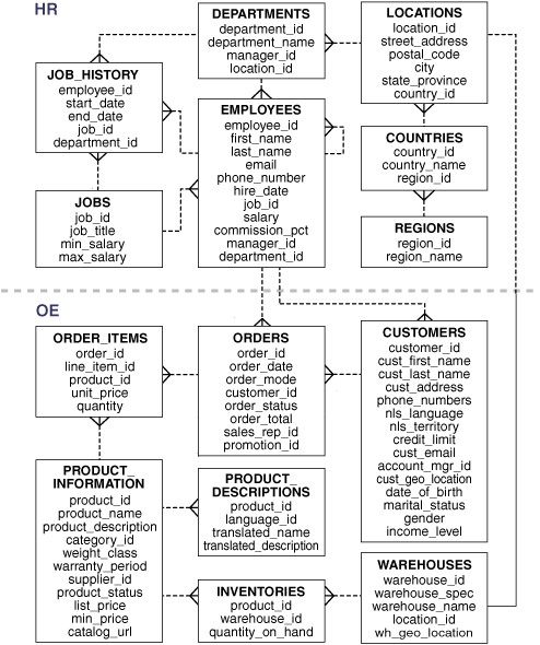
Oracle sample schema OE (Order Entry)
Obviously the database isn’t a native graph engine. If you need more advanced features for analysing your graph it could easily be loaded into PGX. Parallel Graph AnalytiX (PGX) is a toolkit for graph analysis, which also include a single-node in-memory engine or a distributed engine for extremely large graphs. We will look at this aspect in future blog posts.
Create the graph
First thing first is obviously to create the graph. Remember that before to do it, you will need to perform a simple configuration to extend the maximum size of varchar columns (required by the graph solution) and get your DB ready for graphs.
Zhe “Alan” Wu blogged about the steps to get the database ready for graphs, you can find his post at https://blogs.oracle.com/oraclespatial/graph-database-says-hello-from-the-cloud-part-iii.
One of the main requirements is to switch the max string size from standard to extended, which means a varchar could be up to 32’767 bytes instead of the standard 4’000. You can read more about this setting in the documentation.
The creation of the graph couldn’t be simpler than what it is: a single call to opg_apis.create_pg :
|
1 2 3 |
BEGIN OPG_APIS.CREATE_PG('oesample', 4, 8, ''); END; |
First parameter is the name of the graph, second one is the degree or parallelism and the others are defaults (look at the linked doc for the details). The degree of parallelism (DOP) for me is, keeping things simple, the total number of threads available in the system as I want to use as much resources as possible to make things faster (1 CPU with 2 cores with 2 threads each = 1 * 2 * 2 = 4).
After this command you will see, in the schema you used to execute the creation of the graph, some extra tables, the result of the CREATE_PG command.
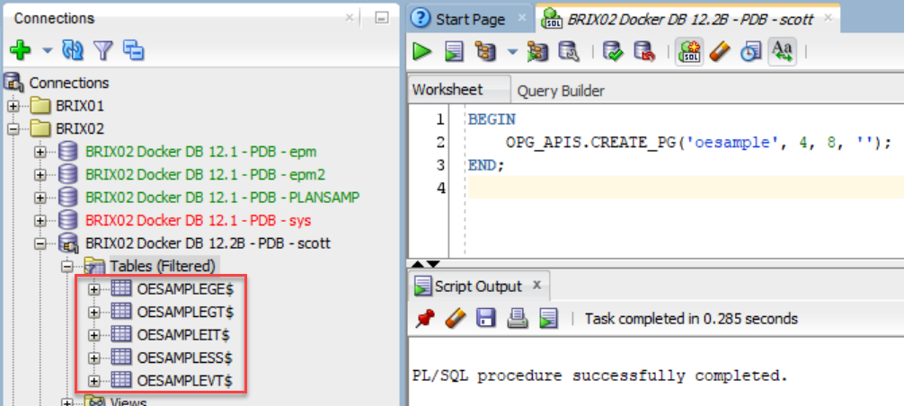
Create a graph by SQL: 1 command and 5 tables are created
The 5 tables created are named with the graph name and a suffix:
- GE$ : edges of the graph
- VT$ : vertices (nodes) of the graph
- GT$ : graph skeleton
- IT$ : text index metadata
- SS$ : graph snapshots
Keeping it really simple you can have a graph by simply focusing on the GE$ and VT$ tables and ignoring the others. For this example it’s what I will do as the other 3 tables are for different and more advanced usages.
Graph tables structure
The structure of the vertices and edges tables is quite simple as the number of columns is limited. To make it easier I added comments to each column describing what its role is (so don’t be surprised if your tables will not have a single comment, it’s normal).

Graph table for vertices, the comments describe each column

Graph table for edges, the comments describe each column
A graph stored in the database using the VT$ and GE$ tables uses the PG / FLAT-FILE format and has the following specifications: vertices IDs as integer or long, vertices labels aren’t supported, edges IDs as long, edges label is supported but a single one per edge.
One of the few things to pay attention at is the property type and its value for both edges and vertices: this is a 100% graph thing. The type is a number telling the graph what data type is the value of the given property, the list of options is available in the PGX documentation (https://docs.oracle.com/cd/E56133_01/latest/reference/loader/file-system/plain-text-formats.html).

List of values for various properties types as visible in the PGX documentation
A given property in a graph must have a unique and single type. Nothing makes that check in the database structure, but that’s how graphs works, so make sure to not mix types for the same property (a same property name in edges and vertices with different types is possible as it relate to different objects).
Once the type is set the value of the property need to be stored in the “V” column if it’s a string. Double stored in the “V” (the string version of it) and “VN” if it is a numeric value, respectively “VT” if it is a date-time value. In this way, with the double storage, the original value is preserved (for calculations and algorithms) and a textual version is available and easy to display without having to pay too much attention at the type and performing transformation or casting.
Create vertices (nodes) by SQL
We saw above the structure of the vertices table, an ID and if needed properties for a vertex. To create a vertex we simply need to insert data into the table respecting that rule. The vertex ID need to be unique but repeated for all the rows with different properties which are related to the same graph vertex (there is a unique constraint on VID-K).
In this example I will create vertices for the customers and products of the OE sample schema as the graph will represent orders passed by customers (so a customer order one or many products: customers and products are vertices, orders will be edges in the graph connection the user and the product ordered).
I wrote a simple query taking some properties of the customers and products and transforming them into vertices. As the customer ID and product ID in the database are already unique, I can use them directly as vertex ID instead of creating a new unique sequence. (double click to see the full code)
|
1 2 3 4 5 6 7 8 9 10 11 12 13 14 15 16 17 18 19 20 21 22 23 24 25 |
INSERT INTO OESAMPLEVT$ (VID, K, T, V, VN, VT) WITH cust AS ( SELECT customer_id AS vid, 'customer_id' AS k, 2 AS t, to_nchar(customer_id) AS v, customer_id AS vn, NULL AS vt FROM oe.customers UNION ALL SELECT customer_id AS vid, 'src_table' AS k, 1 AS t, to_nchar('oe.customers') AS v, NULL AS vn, NULL AS vt FROM oe.customers UNION ALL SELECT customer_id AS vid, 'name' AS k, |
Create edges by SQL
As edges will represent the orders done by customers and the database store order and order items separately there isn’t an already available column acting as edge ID. But this value can be generated by a simple RANK over the orders and order items lines to preserve the same edge ID over the various properties the edge will have. The source vertex ID will be the customer ID and the destination vertex ID will be the product ID. All the information describing the order, as quantity and amounts, will be stored as edge properties. The main difference between edges and vertices is that edges can have a label, but in this case I will simply have a unique value of “order” as label.
There isn’t a unique constraint on SVID-DVID-K because there can be multiple edges connecting the same customer to the same products if somebody ordered many times a product. But there is a unique constraint on EID-K as a property must be single for each edge ID.
|
1 2 3 4 5 6 7 8 9 10 11 12 13 14 15 16 17 18 19 20 21 22 23 24 25 |
INSERT INTO OESAMPLEGE$ (EID, SVID, DVID, EL, K, T, V, VN, VT) WITH ordlines AS ( SELECT ord.order_id, ord.order_date, ord.order_mode, ord.customer_id, ord.order_status, ord.order_total, orditem.line_item_id, orditem.product_id, orditem.unit_price, orditem.quantity FROM oe.orders ord, oe.order_items orditem WHERE ord.order_id = orditem.order_id ),edges AS ( SELECT NULL AS eid, customer_id AS svid, product_id AS dvid, 'order' AS el, 'order_id' AS k, |
Done! The graph is loaded!
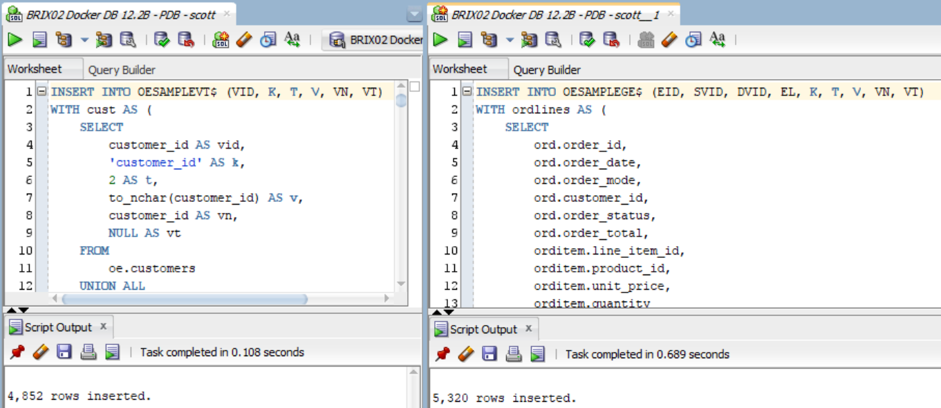
Graph loaded by SQL inserting values in the vertices (VT$) and edges (GE$) tables
Visualize the graph
The graph can be queried by SQL as it is 2 tables which can be joined as required but it can also be used as any other normal Oracle graph. For example a nice and simple way to see the result is by using Cytoscape with the Oracle plugin for graph visualization (http://www.oracle.com/technetwork/database-options/spatialandgraph/downloads/index-156999.html).
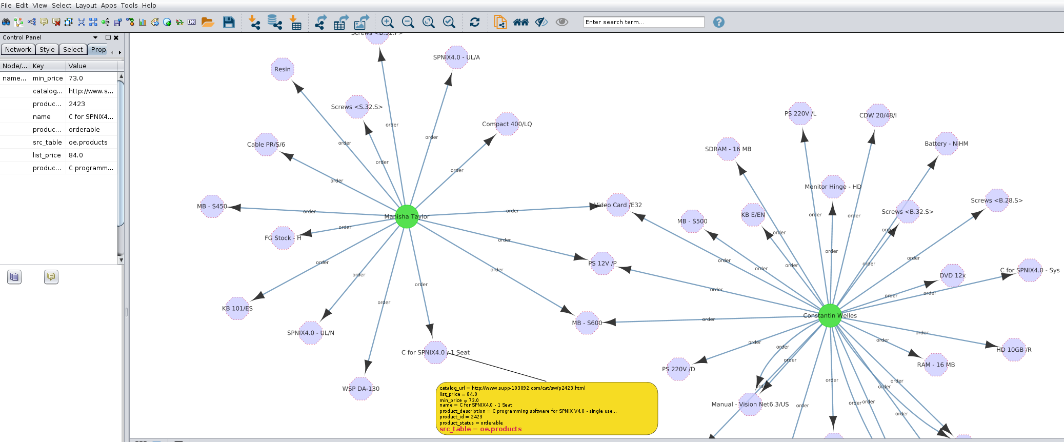
Cytoscape to visualize the graph loaded by SQL
In future blog posts I will go more in details on how to perform analysis on graphs with Cytoscape and PGX. At the moment the number of analysis doable by SQL is limited to counting triangles and page rank. The documentation list all the available methods in the OPG_APIS package and each method come with a simple example making it easy to use.
Run a page rank calculation
Not really the best ever graph for a page rank but let’s see how this kind of calculation can be easily done by SQL. There are 2 methods in the OPG_APIS package, one to prepare the calculation of the page rank and one doing the actual calculation. The output of the preparation is important as it shows values which will be needed at the end to clean up the page rank calculation, so keep a note of the values returned.
|
1 2 3 4 5 6 7 8 9 10 11 12 13 14 15 16 |
SET SERVEROUTPUT ON DECLARE wt_pr varchar2(2000); -- name of the table to hold PR value of the current iteration wt_npr varchar2(2000); -- name of the table to hold PR value for the next iteration wt3 varchar2(2000); wt4 varchar2(2000); wt5 varchar2(2000); n_vertices number; BEGIN wt_pr := 'oesample'; opg_apis.pr_prep('oesampleGE$', wt_pr, wt_npr, wt3, wt4, null); dbms_output.put_line('Working table names ' || wt_pr || ', wt_npr ' || wt_npr || ', wt3 ' || wt3 || ', wt4 '|| wt4); opg_apis.pr('oesampleGE$', 0.85, 10, 0.01, 4, wt_pr, wt_npr, wt3, wt4, 'SYSAUX', null, n_vertices); END; |

Page rank calculation in the database
The page rank is ready to be queried. The result is stored into the table named after the ‘wt_pr’ parameter (“oesample” in my case). The “node” column of the page rank result table is the vertex ID, while the “pr” column is the page rank score.
|
1 2 3 4 5 6 7 8 |
SELECT * FROM oesample ORDER BY pr DESC FETCH FIRST 5 ROWS ONLY; SELECT pr.*, v.* FROM oesample pr , oesampleVT$ v WHERE pr.node = v.vid AND v.k in ('name', 'src_table') ORDER BY pr.pr DESC FETCH FIRST 10 ROWS ONLY; |
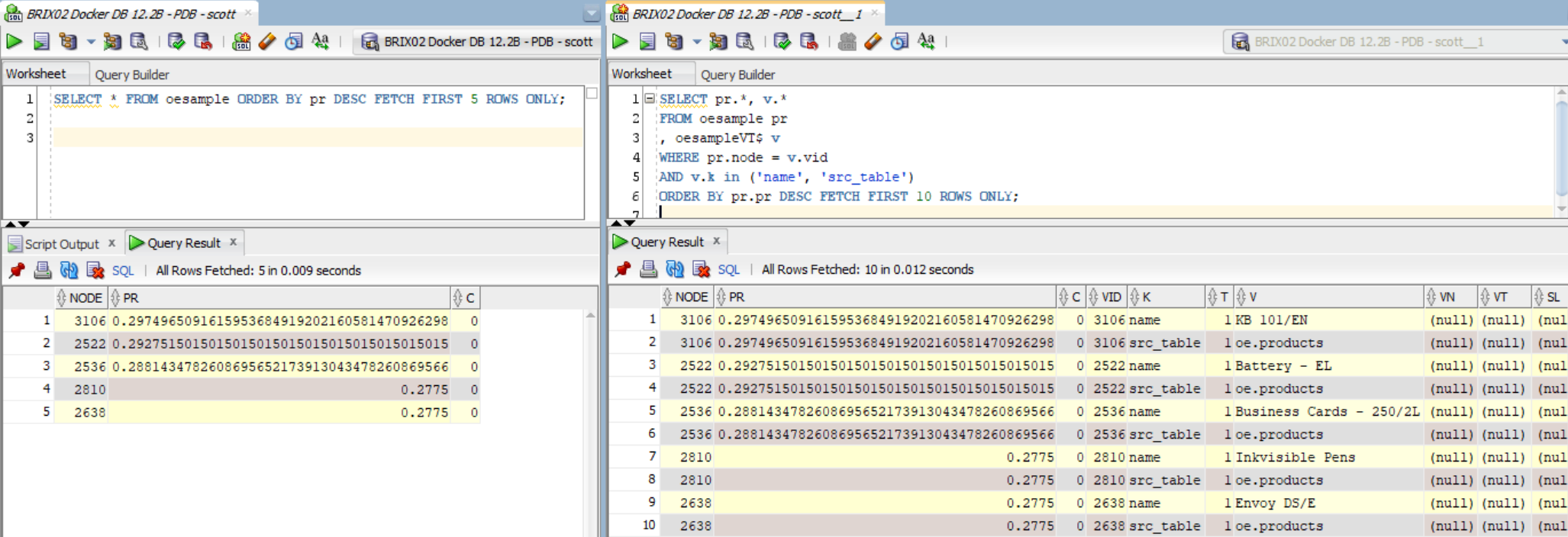
Result of the page rank calculation
Finally once the page rank results aren’t useful anymore it’s time to clean up. Another method exists for that and require the output of the preparation command as arguments.
|
1 2 3 4 5 6 7 8 9 10 11 12 |
DECLARE wt_pr varchar2(2000); -- name of the table to hold PR value of the current iteration wt_npr varchar2(2000); -- name of the table to hold PR value for the next iteration wt3 varchar2(2000); wt4 varchar2(2000); BEGIN wt_pr := 'oesample'; wt_npr := 'OESAMPLEGE$$TWPRX14'; wt3 := 'OESAMPLEGE$$TWPRE14'; wt4 := 'OESAMPLEGE$$TWPRD14'; OPG_APIS.PR_CLEANUP('oesampleGE$', wt_pr, wt_npr, wt3, wt4, null); END; |
The various tables created by page rank have been deleted.
Delete the graph once done
When we are done using the graph we can drop it as easily as we created it.
|
1 2 3 |
BEGIN OPG_APIS.DROP_PG('oesample'); END; |
One single call to DROP_PG passing the graph name as parameter and all the tables and indexes created will all be dropped including all the data.
In just a matter of minutes and by using SQL in SQL Developer we saw how to create, load and drop a graph. It couldn’t be easier than that. No need to write a single line of Java, no need to use Python, no need to use Groovy: just normal SQL.
Stay tuned for more about graphs …
Hi Gianni,
I am not getting any result when executing query
ELECT * FROM oesample ORDER BY pr DESC FETCH FIRST 5 ROWS ONLY;
SELECT pr.*, v.*
FROM oesample pr
, oesampleVT$ v
WHERE pr.node = v.vid
AND v.k in (‘name’, ‘src_table’)
ORDER BY pr.pr DESC FETCH FIRST 10 ROWS ONLY;
I tried 2 times but unable to get the result as shown in the figure ‘Result of the page rank calculation’.
One more thing, How we can create opv & ope files from schema and store in the file path.
Plz help me.
Regards,
Dinesh Gupta
Do you have the table? What is inside? AS this is now a 2 years old post, it’s possible syntax of the package change with versions, did the execution of the procedure go well?